miniTUBA Tutorial

 

For PDF version of this tutorial, click here.

 

miniTUBA is a web-based modeling system that allows clinical and biomedical researchers to perform complex medical/clinical inference and prediction using dynamic Bayesian network analysis with temporal datasets. The software allows users to continuously update their data and refine their results. miniTUBA can make temporal predictions to suggest interventions based on an automated learning process pipeline using all data provided. A detailed step-by-step walk through is provided as follows.  

 

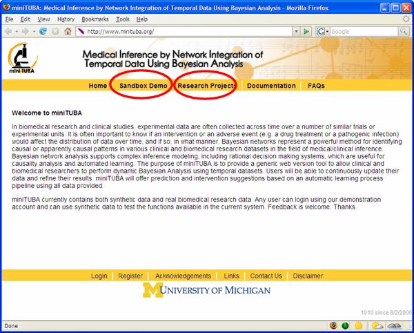
1.         Get started

Point your browser to http://www.minituba.org as shown in Figure 1. To start your own research project, click on “Research Projects”.  To test all the features in miniTUBA using our demo account, click on "Sandbox Demo".

Differences between “Demo” & “Research Projects”: (1) “Research Projects” need individual account. (2) “Research Projects” need approval. (3) “Demo” projects are public, no privacy.

 

Figure 1

 

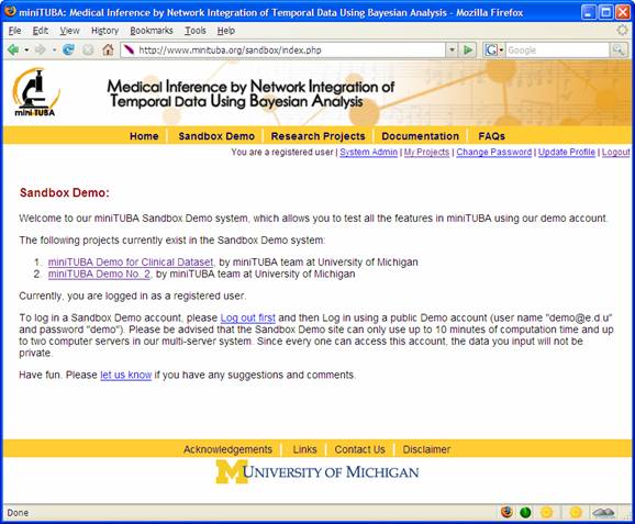
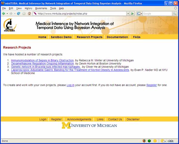
The "Sandbox Demo" (Figure 2) or “Research Projects” (Figure 3) web page lists many projects publicly viewable:

Figure 2

 

 

Figure 3

 

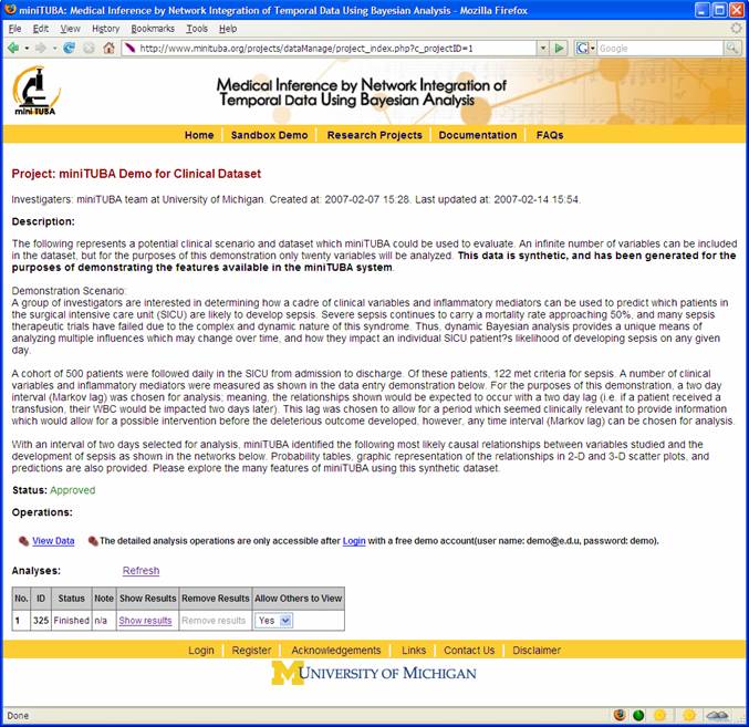
Each project shown in the "Sandbox Demo" or “Research Projects” web page is described (Figure 4). However, the project owner may decide not to show all the operations.

Figure 4

 

2.         Register your account:

 

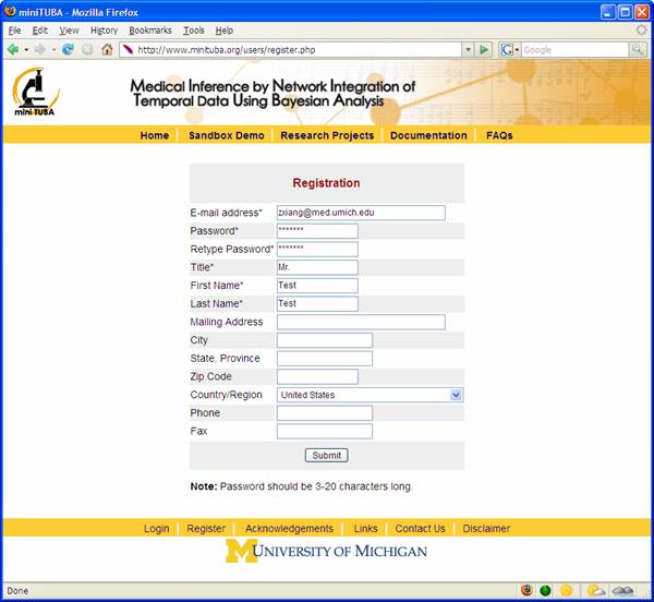
Before setting up your own research project, you need to register an account in miniTUBA and login to our system. To register, click “Register” and fill out the form shown in Figure 5. Once your registration is finished, you can log in and start to create your new project.

NOTE: You don’t need to register for an account if you just want to test the features using our “Sandbox Demo”. Instead, you can use login with user name "demo@e.d.u" and password "demo".

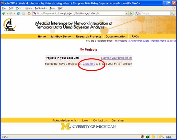
Figure 5

3.         Create your own project

Once logged in, you will see a page listing all of your projects if you have any. You can create a new project as instructed (Figure 6).

 

Figure 6

 

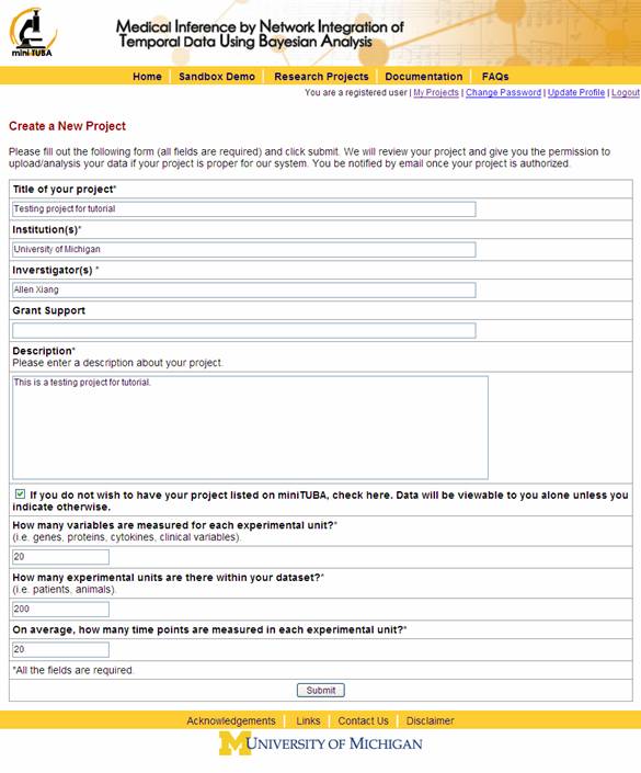
To create a new project, please fill out the form seen in Figure 7.

 

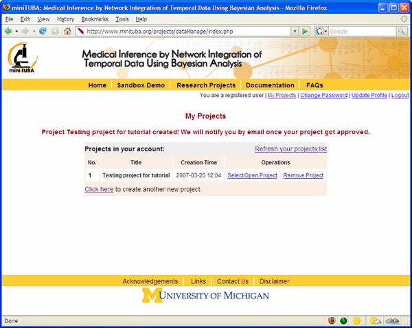
Figure 7

We will review your request and contact you within a few days (Figure 8). NOTE: If you are creating a project in “Sandbox Demo”, your project will be approved automatically.

 

Figure 8

 

Once your project is approved, you can select and open your project by click “Select/Open project” (Figure 8).

 

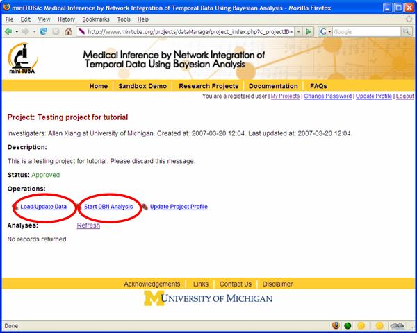
4.         Upload data.

To upload project data, click “Load/Update Data” in Figure 9. 

 

Figure 9

 

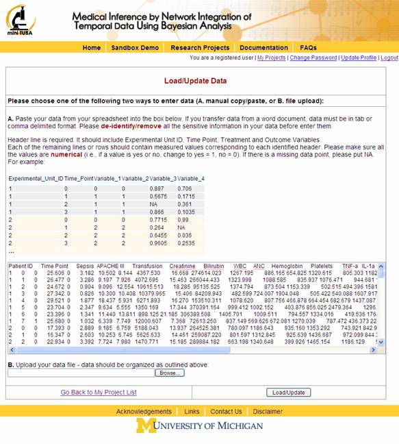
A form will appear and allow you to paste your data into the text box or select the data file you wish to upload (Figure 10).

 

Figure 10

 

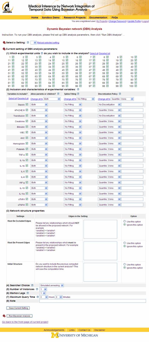
5.         Setting up dynamic Bayesian network analysis parameters

·         Once you have your data uploaded, you can click “Start DBN Analysis” (Figure 9). A form will appear (Figure 11), where you can set up dynamic Bayesian network (DBN) analysis parameters.

Figure 11

NOTES:

 

·         Select a Setting: All settings for each analysis will be stored in our database. You can reload settings from any previous analysis by selecting an analysis and click "Reload selected setting".

 

·         Variables to include: choose variables to include in the analysis.

 

·         Allow parents or children: You can exclude all the relationships start from a variable by select "Parents only", or exclude all the relationships point to a variable by select "Children only"

 

·         Spline Fitting: If you have missing data points for continuous data, spline fitting is required to interpolating those missing data. Spline fitting does NOT work for nominal data.

 

·         Discretization Policy: If the measured values for a variable are continuous, discretization is required. For interval discretization the data range of each bin is equal. The number of data values in each bin varies according to the bin range. For quantile discretization each bin receives an equal number of data values. The data range of each bin varies according to the data values it contains. For customized binning, please enter the cutting points separated by semicolon. 3 is the suggested number of bins.

 

·         Must be Excluded Edges: list any relationships that should NOT be allowed.

 

·         Must Be Present Edges: List any relationships that must be included.

 

·         Initial Structure: include any relationships as prior knowledge.

 

·         Searcher Choice: Simulated Annealing and Greedy approaches are two approaches for searching networks.  The Simulated Annealing approach accepts networks based on a stochastic program implementing Metropolis-Hastings. The Greedy approach always searches for networks with better scores. Simulated annealing is the default selection.

 

·         Number of Instances: Number of computer nodes you wish to use.

 

·         Markov Lags: units of time between two time points to be analyzed in this project. For example, for a project with hourly data sets, Markov lag 1 means 1 hour, and Markov lag 2 means 2 hours, etc.

 

·         Maximum Query time: Depending on the number of variables, the total number of time points, and the discretization policy you select, the maximum query time varies. The more variables, time points or bins you have, the longer time you need to specify here.

 

·         Note: You can put some extra note for this analysis.

 

After all parameters are set, click “Run Bayesian Analysis” (Figure 11).

 

6.         Run DBN analysis

 

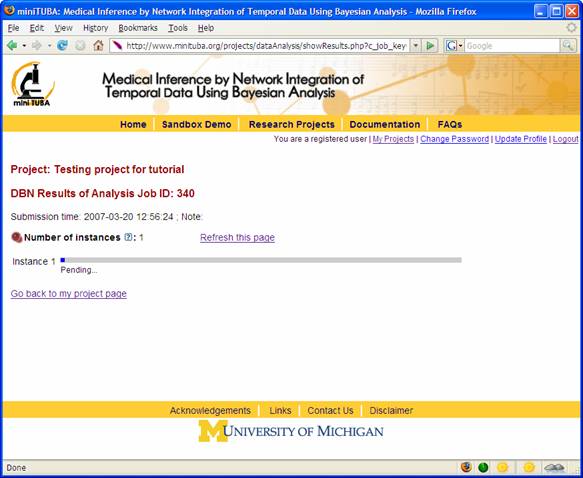
While the dynamic Bayesian nework engine is running, you can periodically check the progress by clicking “Refresh this page” (Figure 12). 

 

Figure 12

 

7.         Check DBN analysis results

 

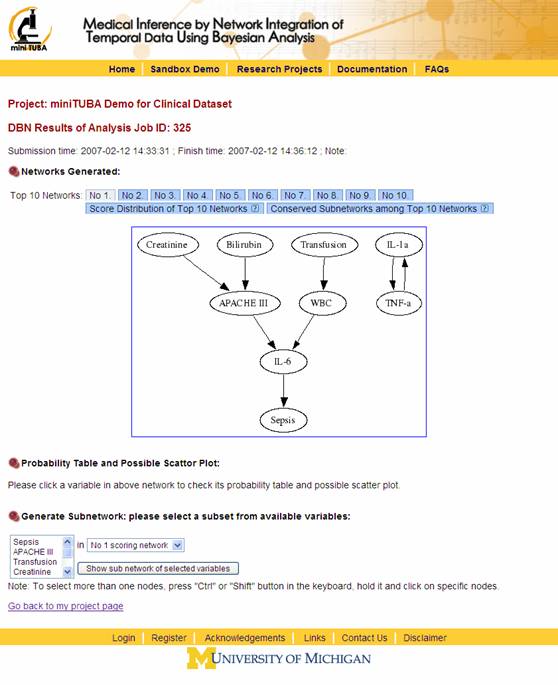
After the DBN analysis is finished, you can check the results (Figure 13).   

 

Figure 13

 

 

·         Top 10 networks: show the top 10 DBN network. Click each one for network display.

 

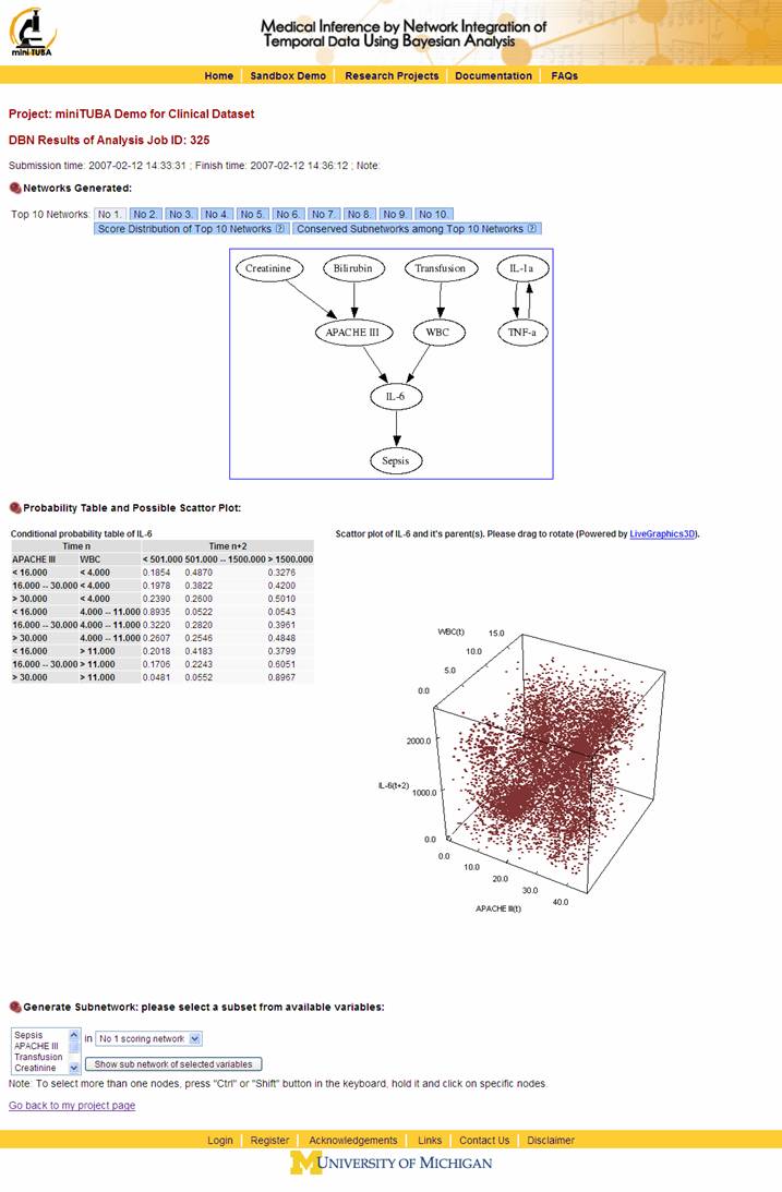
·         Probability Table and Possible Scatter Plot: Click a variable in above network to check its probability table and possible scatter plot.  See Figure 14. For the scatter plot, if it includes three variables, a 3-D image will appear. You can rotate the 3-D image to explore the details.

 

·         Generate Subnetwork: Select a subset of available variables to generate a subset of the above network.

 

 

Figure 14

 

8.         Run prediction

 

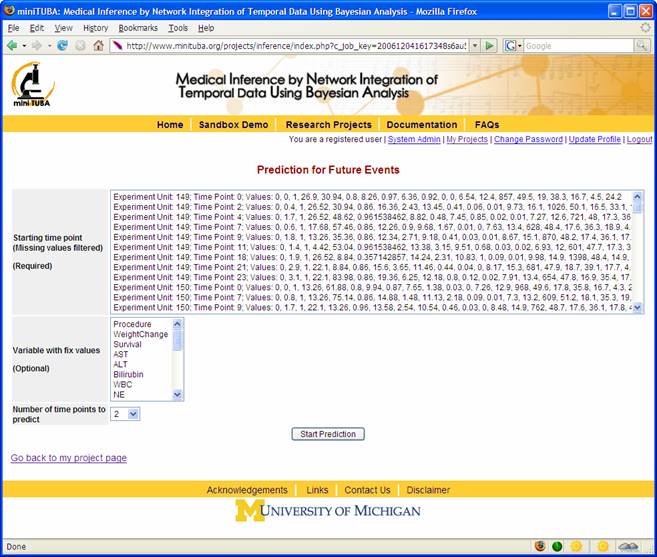
You can also run prediction. You will be prompted to set up the prediction parameters first. See Figure 15. 

Figure 15

 

 

·         Starting time point: It is required to set up a starting time point for future prediction. Any time point with missing data can not be selected.

 

·         Variable with fix values: Select variables with fixed values. The miniTUBA predictin engine will not predict any value for these variables. This is optional.

 

·         Number of time points to predict: select the number of time points to be predicted.

 

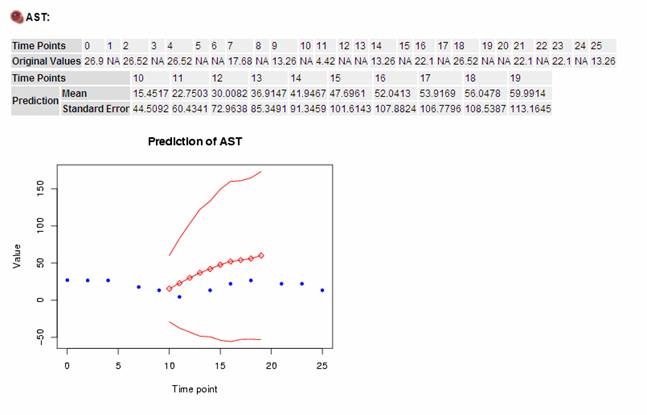
Figure 16

 

One example of prediction results is shown in Figure 16.

 

Suggestions and comments are welcome. Thank you!